Expected output
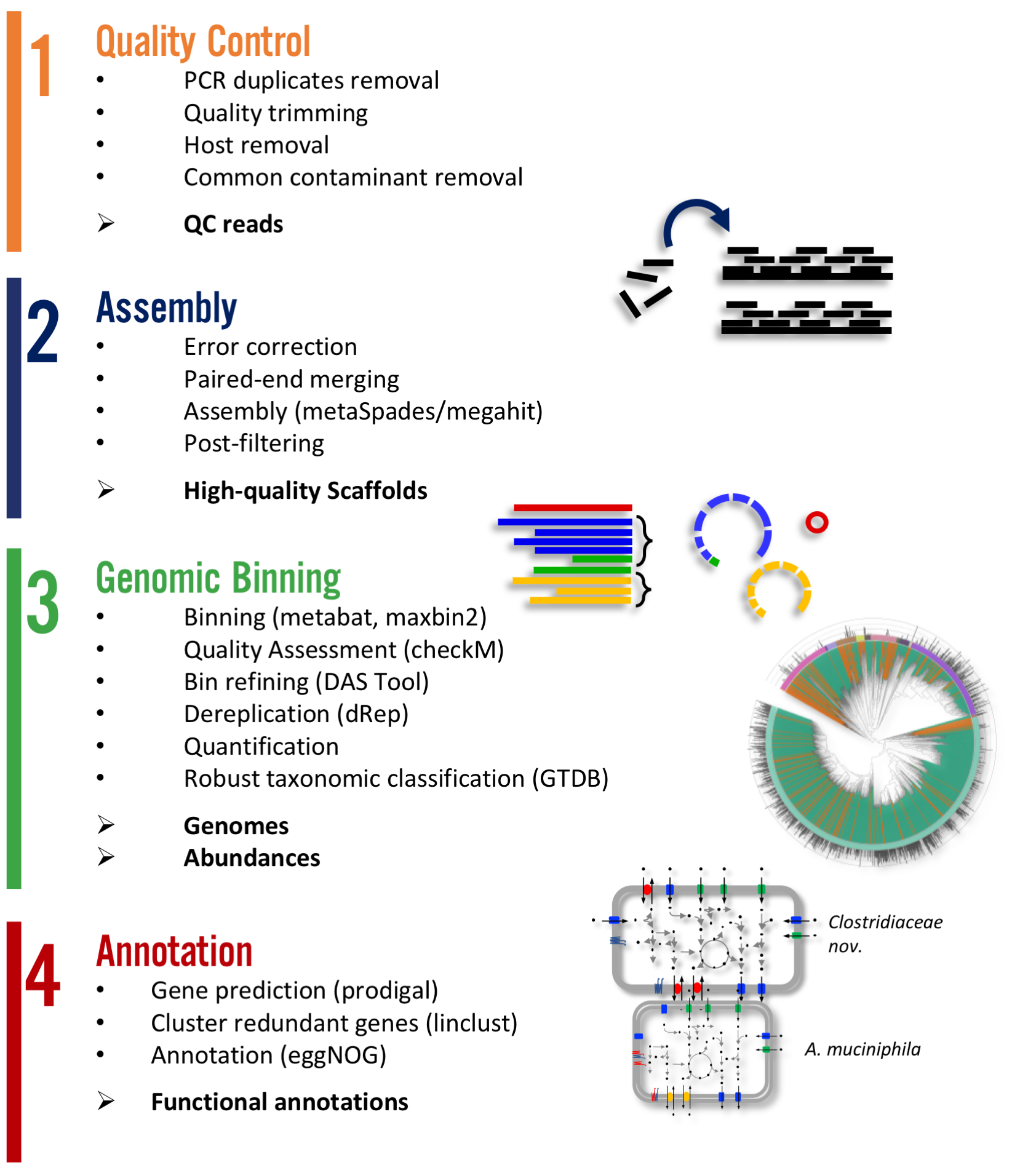
There are two main workflows implemented in atlas. A. Genomes and B. Genecatalog. The first aims in producing metagenome assembled genomes (MAGs) where as the later produces a gene catalog. The steps of Quality control and and
Note
Have a look at the example output at https://github.com/metagenome-atlas/Tutorial/Example .
Quality control
atlas run qc
# or
atlas run genomes
# or
atlas run genecatalog
Runs quality control of single or paired end reads and summarizes the main QC stats in reports/QC_report.html.
Per sample it generates:
{sample}/sequence_quality_control/{sample}_QC_{fraction}.fastq.gz- Various quality stats in
sample}/sequence_quality_control/read_stats
Fractions:
When the input was paired end, we will put out three the reads in three fractions R1,R2 and se The se are the paired end reads which lost their mate during the filtering.
The se reads are no longer used as they usually represent an insignificant number of reads.
Assembly
atlas run assembly
#or
atlas run genomes
# or
atlas run genecatalog
Besides the reports/assembly_report.html this rule outputs the following files per sample:
{sample}/{sample}_contigs.fasta{sample}/sequence_alignment/{sample}.bam{sample}/assembly/contig_stats/final_contig_stats.txt
Binning
atlas run binning
#or
atlas run genomes
When you use different binners (e.g. metabat, maxbin) and a bin-reconciliator (e.g. DAS Tool), then Atlas will produce for each binner and sample:
{sample}/binning/{binner}/cluster_attribution.tsv
which shows the attribution of contigs to bins. For the final_binner it produces the
reports/bin_report_{binner}.html
See an example as a summary of the quality of all bins.
See also
In version 2.8 the new binners vamb and SemiBin were added. First experience show that they outperform the default binner (metabat, maxbin + DASTool). They use a new approach of co-binning which uses the co-abundance from different samples. For more information see the detailed explanation here on page 14
Note
Keep also in mind that maxbin, DASTool, and SemiBin are biased for prokaryotes. If you want to try to bin (small) Eukaryotes use metabat or vamb. More information about Eukaryotes see the discussion here.
Genomes
atlas run genomes
Binning can predict several times the same genome from different samples. To remove this reduncancy we use DeRep to filter and de-replicate the genomes. By default the threshold is set to 97.5%, which corresponds somewhat to the sub-species level. The best quality genome for each cluster is choosen as the representative for each cluster. The represenative MAG are then renamed and used for annotation and quantification.
The fasta sequence of the dereplicated and renamed genomes can be found in genomes/genomes
and their quality estimation are in genomes/checkm/completeness.tsv.
Quantification
The quantification of the genomes can be found in:
genomes/counts/median_coverage_genomes.tsvgenomes/counts/raw_counts_genomes.tsv
See also
See in Atlas example how to analyze these abundances.
Annotations
The annotation can be turned of and on in the config file:
annotations:
  - genes
  - gtdb_tree
  - gtdb_taxonomy
  - kegg_modules
  - dram
The genes option produces predicted genes and translated protein sequences which are stored in genomes/annotations/genes.
Taxonomic adnnotation
A taxonomy for the genomes is proposed by the Genome Taxonomy database (GTDB).
The results can be found in genomes/taxonomy.
The genomes are placed in a phylogenetic tree separately for bacteria and archaea using the GTDB markers.
In addition a tree for bacteria and archaea can be generated based on the checkm markers.
All trees are properly rooted using the midpoint. The files can be found in genomes/tree
Functional annotation
Sicne version 2.8, We use DRAM to annotate the genomes with Functional annotations, e.g. KEGG and CAZy as well as to infere pathways, or more specifically Kegg modules.
The Functional annotations for each genome can be found in genomes/annotations/dram/
and are contain the following files:
kegg_modules.tsvTable of all Kegg modulesannotations.tsvTable of all annotationsdistil/metabolism_summary.xlsxExcel of the summary of all annotationsThe tool alos produces a nice report in distil/product.html.
Gene Catalog
atlas run all
# or
atlas run genecatalog
The gene catalog takes all genes predicted from the contigs and clusters them according to the configuration. It quantifies them by simply mapping reads to the genes (cds sequences) and annotates them using EggNOG mapper.
This rule produces the following output file for the whole dataset.
Genecatalog/gene_catalog.fnaGenecatalog/gene_catalog.faaGenecatalog/annotations/eggNog.tsv.gzGenecatalog/counts/
- Since version 2.15 the output of the quantification are stored in 2 hdf-files`in the folder
Genecatalog/counts/: median_coverage.h5Nmapped_reads.h5.fna
- Together with the statistics per gene and per sample.
gene_coverage_stats.parquetsample_coverage_stats.tsv
The hdf only contains a matrix of abundances or counts under the name data. The sample names are stored as attributes.
The gene names (e.g. Gene00001) are simply the row number.
You can open the hdf file in R or python as following:
import h5py

filename = "path/to/atlas_dir/Genecatalog/counts/median_coverage_genomes.h5"

with h5py.File(filename, 'r') as hdf_file:

    data_matrix = hdf_file['data'][:]
    sample_names = hdf_file['data'].attrs['sample_names'].astype(str)
library(rhdf5)


filename = "path/to/atlas_dir/Genecatalog/counts/median_coverage_genomes.h5"

data <- h5read(filename, "data")

attributes= h5readAttributes(filename, "data")

colnames(data) <- attributes$sample_names
You don’t need to load the full data.
You could only select a subset of genes, e.g. the genes with annotations, or genes that are not singletons.
To find out which gene is a singleton or not you can use the file gene_coverage_stats.parquet
library(rhdf5)
library(dplyr)
library(tibble)

# read only subset of data
indexes_of_genes_to_load = c(2,5,100,150) # e.g. genes with annotations
abundance_file <- file.path(atlas_dir,"Genecatalog/counts/median_coverage.h5")


# get dimension of data

h5overview=h5ls(abundance_file)
dim= h5overview[1,"dim"] %>% stringr::str_split(" x ",simplify=T) %>% as.numeric
cat("Load ",length(indexes_of_genes_to_load), " out of ", dim[1] , " genes\n")


data <- h5read(file = abundance_file, name = "data",
                index = list(indexes_of_genes_to_load, NULL))

# add sample names
attributes= h5readAttributes(abundance_file, "data")
colnames(data) <- attributes$sample_names


# add gene names (e.g. Gene00001) as rownames
gene_names = paste0("Gene", formatC(format="d",indexes_of_genes_to_load,flag="0",width=ceiling(log10(max(dim[1])))))
rownames(data) <- gene_names


data[1:5,1:5]
If you do this you can use the information in the file Genecatalog/counts/sample_coverage_stats.tsv to normalize the counts.
Here is the R code to calculate the gene copies per million (analogous to transcript per million) for the subset of genes.
# Load gene stats per sample
gene_stats_file = file.path(atlas_dir,"Genecatalog/counts/sample_coverage_stats.tsv")

gene_stats <- read.table(gene_stats_file,sep='\t',header=T,row.names=1)

gene_stats <- t(gene_stats) # might be transposed, sample names should be index

head(gene_stats)

# calculate copies per million
total_covarage <- gene_stats[colnames(data)  ,"Sum_coverage"]

# gives wrong results
#gene_gcpm<- data / total_covarage *1e6

gene_gcpm<- data %*% diag(1/total_covarage) *1e6
colnames(gene_gcpm) <- colnames(data)

gene_gcpm[1:5,1:5]
See also
See in Atlas Tutorial
Before version 2.15 the output of the counts were stored in a parquet file.
The parquet file can be opended easily with pandas.read_parquet or arrow::read_parquet`.
However you need to load the full data into memory.
parquet_file <- file.path(atlas_dir,"Genecatalog/counts/median_coverage.parquet")
gene_abundances<- arrow::read_parquet(parquet_file)

# transform tibble to a matrix
gene_matrix= as.matrix(gene_abundances[,-1])
rownames(gene_matrix) <- gene_abundances$GeneNr


#calculate copies per million
gene_gcpm= gene_matrix/ colSums(gene_matrix) *1e6


gene_gcpm[1:5,1:5]
All
The option of atlas run all runs both Genecatalog and Genome workflows and creates mapping tables between Genecatalog and Genomes. However, in future the two workflows are expected to diverge more and more to fulfill their aim better.
If you want to run both workflows together you can do this by:
atlas run genomes genecatalog
If you are interested in mapping the genes to the genomes see the discussion at https://github.com/metagenome-atlas/atlas/issues/413